July 18, 2017 · 16 min read

In a previous post ([Using Principal Component Analysis (PCA) for data Explore: Step by Step]), we have introduced the PCA technique as a method for Matrix Factorization. In that publication, we indicated that, when working with Machine Learning for data analysis, we often encounter huge data sets that has possess hundreds or thousands of different features or variables. As a consequence, the size of the space of variables increases greatly, hindering the analysis of the data for extracting conclusions. In order to address this problem, the Matrix Factorization is a simple way to reduce the dimensionality of the space of variables when considering multivariate data.
In this post we introduce another technique for dimensionality reduction to analyze multivariate data sets. In particular, we shall explain how to employ the technique of Linear Discriminant Analysis (LDA) to reduce the dimensionality of the space of variables and compare it with the PCA technique, so that we can have some criteria on which should be employed in a given case.
Linear Discriminant Analysis (LDA) is a generalization of Fisher's linear discriminant, a method used in Statistics, pattern recognition and machine learning to find a linear combination of features that characterizes or separates two or more classes of objects or events. This method projects a dataset onto a lower-dimensional space with good class-separability to avoid overfitting (“curse of dimensionality”), and to reduce computational costs. The resulting combination may be used as a linear classifier or, more commonly, for dimensionality reduction before subsequent classification.
The original Linear discriminant was described for a 2-class problem, and it was then later generalized as “multi-class Linear Discriminant Analysis” or “Multiple Discriminant Analysis” by C. R. Rao in 1948 (The utilization of multiple measurements in problems of biological classification)
In a nutshell, the goal of a LDA is often to project a feature space (a dataset $n$-dimensional samples) into a smaller subspace $k$ (where $ k \leq n−1$), while maintaining the class-discriminatory information. In general, dimensionality reduction does not only help to reduce computational costs for a given classification task, but it can also be helpful to avoid overfitting by minimizing the error in parameter estimation.
Both Linear Discriminant Analysis (LDA) and Principal Component Analysis (PCA) are linear transformation techniques that are commonly used for dimensionality reduction (both are techniques for the data Matrix Factorization). The most important difference between both techniques is that PCA can be described as an “unsupervised” algorithm, since it “ignores” class labels and its goal is to find the directions (the so-called principal components) that maximize the variance in a dataset, while that the LDA is a “supervised” algorithm that computes the directions (“linear discriminants”) representing the axes that maximize the separation between multiple classes.
Intuitively, we might think that LDA is superior to PCA for a multi-class classification task where the class labels are known. However, this might not always be the case. For example, comparisons between classification accuracies for image recognition after using PCA or LDA show that PCA tends to outperform LDA if the number of samples per class is relatively small (PCA vs. LDA, A.M. Martinez et al., 2001). In practice, it is not uncommon to use both LDA and PCA in combination: e.g., PCA for dimensionality reduction followed by LDA.
In a few words, we can say that the PCA is unsupervised algorithm that attempts to find the orthogonal component axes of maximum variance in a dataset ([see our previous post on his topic]), while the goal of LDA as supervised algorithm is to find the feature subspace that optimizes class separability.
In the following figure, we can see a conceptual scheme that helps us to have a geometric notion about of both methods
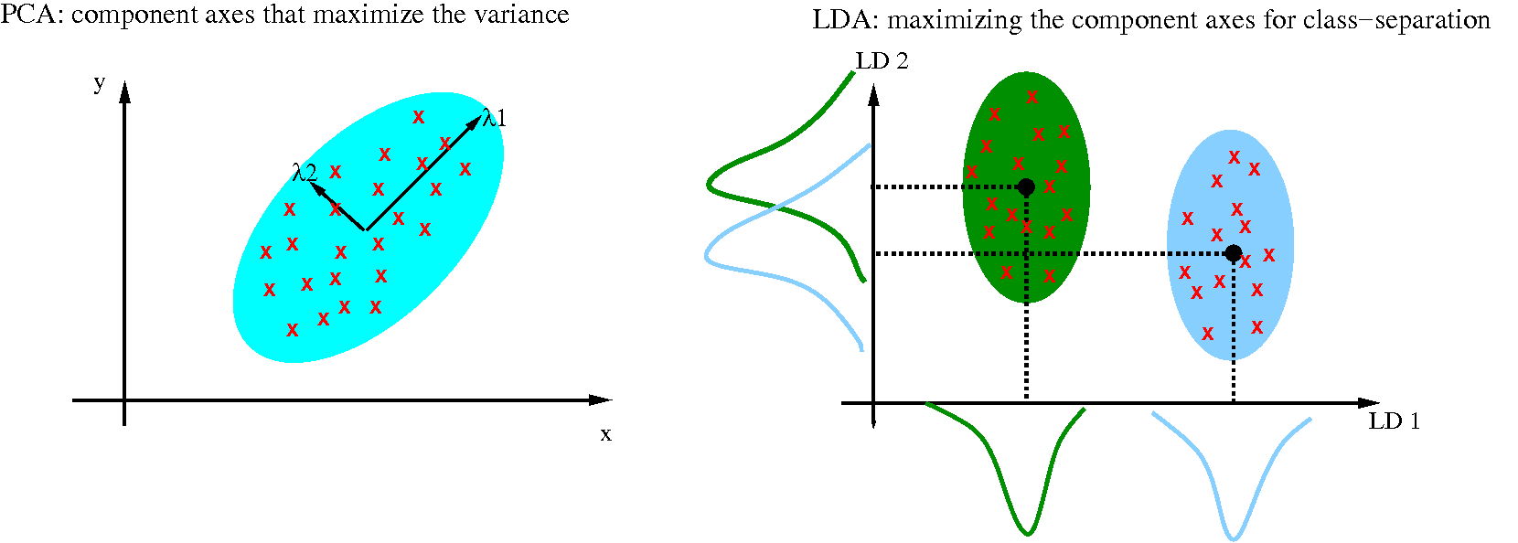
As shown on the x-axis (LD 1 new component in the reduced dimensionality) and y-axis (LD 2 new component in the reduced dimensionality) in the right side of the previous figure, LDA would separate the two normally distributed classes well.
The next question is: What is a “good” feature subspace that maximizing the component axes for class-separation ?
To answer this question, let’s assume that our goal is to reduce the dimensions of a d -dimensional dataset by projecting it onto a (k)-dimensional subspace (where k<d). So, how do we know what size we should choose for k (k = the number of dimensions of the new feature subspace), and how do we know if we have a feature space that represents our data “well”?
For that, we will compute eigenvectors (the components) from our data set and collect them in a so-called scatter-matrices (i.e., the in-between-class scatter matrix and within-class scatter matrix). Each of these eigenvectors is associated with an eigenvalue, which tells us about the “length” or “magnitude” of the eigenvectors.
If we would observe that all eigenvalues have a similar magnitude, then this may be a good indicator that our data is already projected on a “good” feature space.
And in the other scenario, if some of the eigenvalues are much much larger than others, we might be interested in keeping only those eigenvectors with the highest eigenvalues, since they contain more information about our data distribution. The other way, if the eigenvalues that are close to 0 are less informative and we might consider dropping those for constructing the new feature subspace (same procedure that in the case of PCA ).
We listed the 5 general steps for performing a linear discriminant analysis; we will explore them in more detail in the following sections.
Compute the $d-dimensional$ mean vectors for the different classes from the dataset.
Compute the scatter matrices (in-between-class and within-class scatter matrix).
Compute the eigenvectors ($e_1,e_2,...,e_d$) and corresponding eigenvalues ($\lambda_1,\lambda_2,...\lambda_d$) for the scatter matrices.
Sort the eigenvectors by decreasing eigenvalues and choose k eigenvectors with the largest eigenvalues to form a $d \times k$ dimensional matrix $W$ (where every column represents an eigenvector).
Use this $d \times k$ eigenvector matrix to transform the samples onto the new subspace. This can be summarized by the matrix multiplication: $Y=X \times W$, where $X$ is a $n \times d-dimensional $ matrix representing the $n$ samples, and $y$ are the transformed $n \times k-dimensional$ samples in the new subspace.
In order to fixed the concepts we apply this 5 steps in the iris dataset for flower classification.
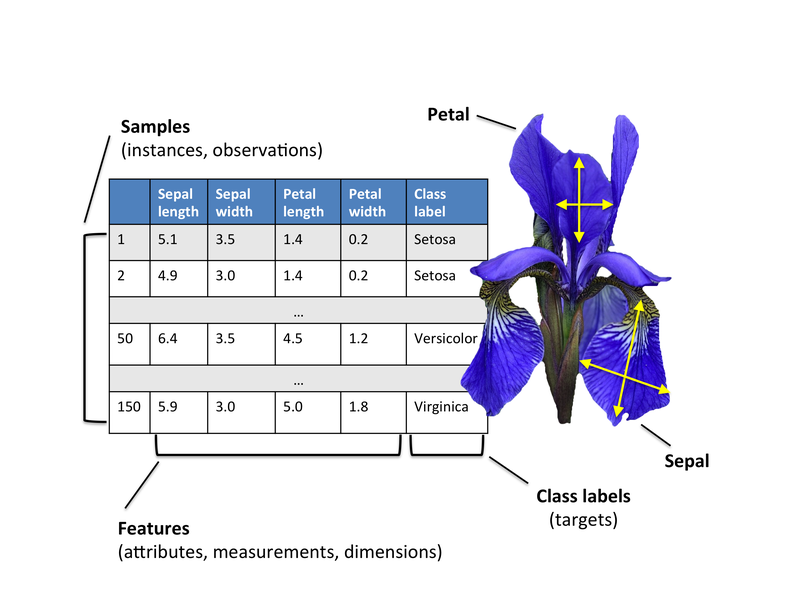
For the following tutorial, we will be working with the famous “Iris” dataset that has been deposited on the UCI machine learning repository (https://archive.ics.uci.edu/ml/datasets/Iris).
The iris dataset contains measurements for 150 iris flowers from three different species.
The three classes in the Iris dataset:
The four features of the Iris dataset:
feature_dict = {i:label for i,label in zip(
                range(4),
                  ('sepal length in cm',
                  'sepal width in cm',
                  'petal length in cm',
                  'petal width in cm', ))}
Reading in the dataset
import pandas as pd

df = pd.io.parsers.read_csv(
    filepath_or_buffer='https://archive.ics.uci.edu/ml/machine-learning-databases/iris/iris.data',
    header=None,
    sep=',',
    )
df.columns = [l for i,l in sorted(feature_dict.items())] + ['class label']
df.dropna(how="all", inplace=True) # to drop the empty line at file-end

df.tail()
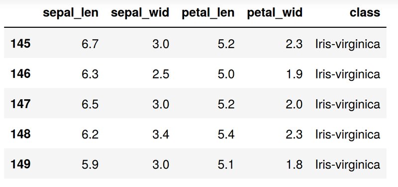
In matrix form
$ \mathbf{X} = \begin{bmatrix} x_{1_{\text{sepal length}}} & x_{1_{\text{sepal width}}} & x_{1_{\text{petal length}}} & x_{1_{\text{petal width}}} \newline ... \newline x_{2_{\text{sepal length}}} & x_{2_{\text{sepal width}}} & x_{2_{\text{petal length}}} & x_{2_{\text{petal width}}} \newline \end{bmatrix}, y = \begin{bmatrix} \omega_{\text{iris-setosa}}\newline ... \newline \omega_{\text{iris-virginica}}\newline \end{bmatrix}$
Since it is more convenient to work with numerical values, we will use the LabelEncode from the scikit-learn library to convert the class labels into numbers: 1, 2, and 3.
%matplotlib inline

from sklearn.preprocessing import LabelEncoder

X = df[[0,1,2,3]].values
y = df['class label'].values

enc = LabelEncoder()
label_encoder = enc.fit(y)
y = label_encoder.transform(y) + 1

label_dict = {1: 'Setosa', 2: 'Versicolor', 3:'Virginica'}
We obtain
$y = \begin{bmatrix}{\text{setosa}}\newline {\text{setosa}}\newline ... \newline {\text{virginica}}\end{bmatrix} \quad \Rightarrow \begin{bmatrix} {\text{1}}\ {\text{1}} \newline ... \newline {\text{3}}\end{bmatrix}$
Just to get a rough idea how the samples of our three classes $\omega_1, \omega_2$ and $\omega_3$ are distributed, let us visualize the distributions of the four different features in 1-dimensional histograms.
%matplotlib inline

from matplotlib import pyplot as plt
import numpy as np
import math

fig, axes = plt.subplots(nrows=2, ncols=2, figsize=(12,6))

for ax,cnt in zip(axes.ravel(), range(4)):

    # set bin sizes
    min_b = math.floor(np.min(X[:,cnt]))
    max_b = math.ceil(np.max(X[:,cnt]))
    bins = np.linspace(min_b, max_b, 25)

    # plottling the histograms
    for lab,col in zip(range(1,4), ('blue', 'red', 'green')):
        ax.hist(X[y==lab, cnt],
                   color=col,
                   label='class %s' %label_dict[lab],
                   bins=bins,
                   alpha=0.5,)
    ylims = ax.get_ylim()

    # plot annotation
    leg = ax.legend(loc='upper right', fancybox=True, fontsize=8)
    leg.get_frame().set_alpha(0.5)
    ax.set_ylim([0, max(ylims)+2])
    ax.set_xlabel(feature_dict[cnt])
    ax.set_title('Iris histogram #%s' %str(cnt+1))

    # hide axis ticks
    ax.tick_params(axis="both", which="both", bottom="off", top="off",
            labelbottom="on", left="off", right="off", labelleft="on")

    # remove axis spines
    ax.spines["top"].set_visible(False)
    ax.spines["right"].set_visible(False)
    ax.spines["bottom"].set_visible(False)
    ax.spines["left"].set_visible(False)

axes[0][0].set_ylabel('count')
axes[1][0].set_ylabel('count')

fig.tight_layout()

plt.show()
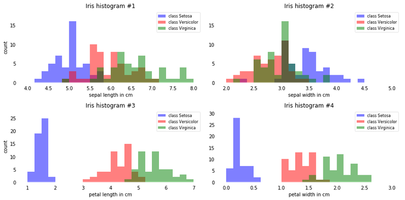
From just looking at these simple graphical representations of the features, we can already tell that the petal lengths and widths are likely better suited as potential features two separate between the three flower classes. In practice, instead of reducing the dimensionality via a projection (here: LDA), a good alternative would be a feature selection technique. For low-dimensional datasets like Iris, a glance at those histograms would already be very informative. Another simple, but very useful technique would be to use feature selection algorithms (see rasbt.github.io/mlxtend/user_guide/feature_selection/SequentialFeatureSelector and scikit-learn).
Important note about of normality assumptions: It should be mentioned that LDA assumes normal distributed data, features that are statistically independent, and identical covariance matrices for every class. However, this only applies for LDA as classifier and LDA for dimensionality reduction can also work reasonably well if those assumptions are violated. And even for classification tasks LDA seems can be quite robust to the distribution of the data.
After we went through several preparation steps, our data is finally ready for the actual LDA. In practice, LDA for dimensionality reduction would be just another preprocessing step for a typical machine learning or pattern classification task.
In this first step, we will start off with a simple computation of the mean vectors $m_i$, $(i=1,2,3)$ of the 3 different flower classes:
$ m_i = \begin{bmatrix} \mu_{\omega_i (\text{sepal length)}}\newline \mu_{\omega_i (\text{sepal width})}\newline \mu_{\omega_i (\text{petal length)}}\newline \mu_{\omega_i (\text{petal width})}\newline \end{bmatrix} \; , \quad \text{with} \quad i = 1,2,3$
np.set_printoptions(precision=4)

mean_vectors = []
for cl in range(1,4):
    mean_vectors.append(np.mean(X[y==cl], axis=0))
    print('Mean Vector class %s: %s\n' %(cl, mean_vectors[cl-1]))
we obtain:
   Mean Vector class 1: [ 5.006  3.418  1.464  0.244]

   Mean Vector class 2: [ 5.936  2.77   4.26   1.326]

   Mean Vector class 3: [ 6.588  2.974  5.552  2.026]
Now, we will compute the two 4x4-dimensional matrices: The within-class and the between-class scatter matrix.
The within-class scatter matrix SW is computed by the following equation:
$ S_W = \sum\limits_{i=1}^{c} S_i$
where
$ S_i = \sum\limits_{\pmb x \in D_i}^n (\pmb x - \pmb m_i)\;(\pmb x - \pmb m_i)^T $
and mmi is the mean vector
$ \pmb m_i = \frac{1}{n_i} \sum\limits_{\pmb x \in D_i}^n \; \pmb x_k$
S_W = np.zeros((4,4))
for cl,mv in zip(range(1,4), mean_vectors):
    class_sc_mat = np.zeros((4,4))                  # scatter matrix for every class
    for row in X[y == cl]:
        row, mv = row.reshape(4,1), mv.reshape(4,1) # make column vectors
        class_sc_mat += (row-mv).dot((row-mv).T)
    S_W += class_sc_mat                             # sum class scatter matrices
print('within-class Scatter Matrix:\n', S_W)
we obtain:
within-class Scatter Matrix:
 [[ 38.9562  13.683   24.614    5.6556]
 [ 13.683   17.035    8.12     4.9132]
 [ 24.614    8.12    27.22     6.2536]
 [  5.6556   4.9132   6.2536   6.1756]]
2.1 b
Alternatively, we could also compute the class-covariance matrices by adding the scaling factor $\frac{1}{N−1}$ to the within-class scatter matrix, so that our equation becomes
$\Sigma_i = \frac{1}{N_{i}-1} \sum\limits_{\pmb x \in D_i}^n (\pmb x - \pmb m_i)\;(\pmb x - \pmb m_i)^T$
and
$S_W = \sum\limits_{i=1}^{c} (N_{i}-1) \Sigma_i$
where $N_i$ is the sample size of the respective class (here: 50), and in this particular case, we can drop the term ($N_i−1$) since all classes have the same sample size.
However, the resulting eigenspaces will be identical (identical eigenvectors, only the eigenvalues are scaled differently by a constant factor).
2.2 Between-class scatter matrix $S_B$
The between-class scatter matrix $S_B$ is computed by the following equation:
$S_B = \sum\limits_{i=1}^{c} N_{i} (\pmb m_i - \pmb m) (\pmb m_i - \pmb m)^T$
where $m$ is the overall mean, and mmi and $N_i$ are the sample mean and sizes of the respective classes.
overall_mean = np.mean(X, axis=0)

S_B = np.zeros((4,4))
for i,mean_vec in enumerate(mean_vectors):
    n = X[y==i+1,:].shape[0]
    mean_vec = mean_vec.reshape(4,1) # make column vector
    overall_mean = overall_mean.reshape(4,1) # make column vector
    S_B += n * (mean_vec - overall_mean).dot((mean_vec - overall_mean).T)

print('between-class Scatter Matrix:\n', S_B)
We obtain
between-class Scatter Matrix:
 [[  63.2121  -19.534   165.1647   71.3631]
 [ -19.534    10.9776  -56.0552  -22.4924]
 [ 165.1647  -56.0552  436.6437  186.9081]
 [  71.3631  -22.4924  186.9081   80.6041]]
Next, we will solve the generalized eigenvalue problem for the matrix $S_{W}^{-1} S_{B}$ to obtain the linear discriminants.
eig_vals, eig_vecs = np.linalg.eig(np.linalg.inv(S_W).dot(S_B))

for i in range(len(eig_vals)):
    eigvec_sc = eig_vecs[:,i].reshape(4,1)
    print('\nEigenvector {}: \n{}'.format(i+1, eigvec_sc.real))
    print('Eigenvalue {:}: {:.2e}'.format(i+1, eig_vals[i].real))
we obtain
Eigenvector 1:
[[-0.2049]
 [-0.3871]
 [ 0.5465]
 [ 0.7138]]
Eigenvalue 1: 3.23e+01

Eigenvector 2:
[[-0.009 ]
 [-0.589 ]
 [ 0.2543]
 [-0.767 ]]
Eigenvalue 2: 2.78e-01

Eigenvector 3:
[[ 0.179 ]
 [-0.3178]
 [-0.3658]
 [ 0.6011]]
Eigenvalue 3: -4.02e-17

Eigenvector 4:
[[ 0.179 ]
 [-0.3178]
 [-0.3658]
 [ 0.6011]]
Eigenvalue 4: -4.02e-17
After this decomposition of our square matrix into eigenvectors and eigenvalues, let us briefly recapitulate how we can interpret those results. Both eigenvectors and eigenvalues are providing us with information about the distortion of a linear transformation: The eigenvectors are basically the direction of this distortion, and the eigenvalues are the scaling factor for the eigenvectors that describing the magnitude of the distortion.
If we are performing the LDA for dimensionality reduction, the eigenvectors are important since they will form the new axes of our new feature subspace; the associated eigenvalues are of particular interest since they will tell us how “informative” the new “axes” are.
Let us briefly double-check our calculation and talk more about the eigenvalues below.
$\pmb A\pmb{v} = \lambda\pmb{v}$
where, $ \pmb A = S_{W}^{-1}S_B$, $ \pmb {v} = \text{Eigenvector}$ and $\lambda = \text{Eigenvalue}$
for i in range(len(eig_vals)):
    eigv = eig_vecs[:,i].reshape(4,1)
    np.testing.assert_array_almost_equal(np.linalg.inv(S_W).dot(S_B).dot(eigv),
                                         eig_vals[i] * eigv,
                                         decimal=6, err_msg='', verbose=True)
print('ok')
we obtain
ok
Remember from the introduction that we are not only interested in merely projecting the data into a subspace that improves the class separability, but also reduces the dimensionality of our feature space, (where the eigenvectors will form the axes of this new feature subspace).
However, the eigenvectors only define the directions of the new axis, since they have all the same unit length 1.
So, in order to decide which eigenvector(s) we want to drop for our lower-dimensional subspace, we have to take a look at the corresponding eigenvalues of the eigenvectors. Roughly speaking, the eigenvectors with the lowest eigenvalues bear the least information about the distribution of the data, and those are the ones we want to drop. The common approach is to rank the eigenvectors from highest to lowest corresponding eigenvalue and choose the top $k$ eigenvectors.
# Make a list of (eigenvalue, eigenvector) tuples
eig_pairs = [(np.abs(eig_vals[i]), eig_vecs[:,i]) for i in range(len(eig_vals))]

# Sort the (eigenvalue, eigenvector) tuples from high to low
eig_pairs = sorted(eig_pairs, key=lambda k: k[0], reverse=True)

# Visually confirm that the list is correctly sorted by decreasing eigenvalues

print('Eigenvalues in decreasing order:\n')
for i in eig_pairs:
    print(i[0])
we obtain
Eigenvalues in decreasing order:

32.2719577997
0.27756686384
5.71450476746e-15
5.71450476746e-15
If we take a look at the eigenvalues, we can already see that 2 eigenvalues are close to 0. The reason why these are close to 0 is not that they are not informative but it’s due to floating-point imprecision. In fact, these two last eigenvalues should be exactly zero: In LDA, the number of linear discriminants is at most $c−1$ where $c$ is the number of class labels, since the in-between scatter matrix $S_B$ is the sum of $c$ matrices with rank 1 or less. Note that in the rare case of perfect collinearity (all aligned sample points fall on a straight line), the covariance matrix would have rank one, which would result in only one eigenvector with a nonzero eigenvalue.
Now, let’s express the “explained variance” as percentage:
print('Variance explained:\n')
eigv_sum = sum(eig_vals)
for i,j in enumerate(eig_pairs):
    print('eigenvalue {0:}: {1:.2%}'.format(i+1, (j[0]/eigv_sum).real))
we obtain
Variance explained:

eigenvalue 1: 99.15%
eigenvalue 2: 0.85%
eigenvalue 3: 0.00%
eigenvalue 4: 0.00%
The first eigenpair is by far the most informative one, and we won’t loose much information if we would form a 1D-feature spaced based on this eigenpair.
4.2. Choosing k eigenvectors with the largest eigenvalues
After sorting the eigenpairs by decreasing eigenvalues, it is now time to construct our $k \times d-dimensional$ eigenvector matrix $W$ (here 4×2: based on the 2 most informative eigenpairs) and thereby reducing the initial 4-dimensional feature space into a 2-dimensional feature subspace.
W = np.hstack((eig_pairs[0][1].reshape(4,1), eig_pairs[1][1].reshape(4,1)))
print('Matrix W:\n', W.real)
We obtain
Matrix W:
 [[ 0.2049 -0.009 ]
 [ 0.3871 -0.589 ]
 [-0.5465  0.2543]
 [-0.7138 -0.767 ]]
In the last step, we use the $4 \times 2-dimensional$ matrix $W$ that we just computed to transform our samples onto the new subspace via the equation $Y=X \times W$.
where $X$ is a $ n \times d-dimensional$ matrix representing the $n$ samples, and $Y$ are the transformed $n \times k-dimensional$ samples in the new subspace.
X_lda = X.dot(W)
assert X_lda.shape == (150,2), "The matrix is not 150x2 dimensional."
and we plot the result
from matplotlib import pyplot as plt

def plot_step_lda():

    ax = plt.subplot(111)
    for label,marker,color in zip(
        range(1,4),('^', 's', 'o'),('blue', 'red', 'green')):

        plt.scatter(x=X_lda[:,0].real[y == label],
                y=X_lda[:,1].real[y == label],
                marker=marker,
                color=color,
                alpha=0.5,
                label=label_dict[label]
                )

    plt.xlabel('LD1')
    plt.ylabel('LD2')

    leg = plt.legend(loc='upper right', fancybox=True)
    leg.get_frame().set_alpha(0.5)
    plt.title('LDA: Iris projection onto the first 2 linear discriminants')

    # hide axis ticks
    plt.tick_params(axis="both", which="both", bottom="off", top="off",
            labelbottom="on", left="off", right="off", labelleft="on")

    # remove axis spines
    ax.spines["top"].set_visible(False)
    ax.spines["right"].set_visible(False)
    ax.spines["bottom"].set_visible(False)
    ax.spines["left"].set_visible(False)

    plt.grid()
    plt.tight_layout
    plt.show()

plot_step_lda()
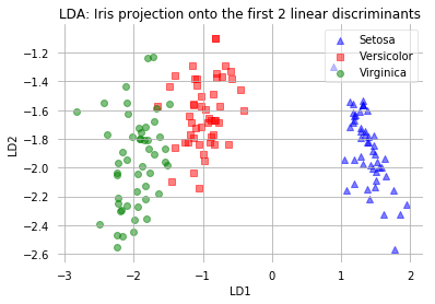
The scatter plot above represents our new feature subspace that we constructed via LDA. We can see that the first linear discriminant “LD1” separates the classes quite nicely. However, the second discriminant, “LD2”, does not add much valuable information, which we’ve already concluded when we looked at the ranked eigenvalues is step 4.
Now, after we have seen how an Linear Discriminant Analysis works using a step-by-step approach, there is also a more convenient way to achive the same via the LDA class implemented in the scikit-learn machine learning library.
# import library

import pandas as pd
from sklearn.preprocessing import LabelEncoder
from sklearn.discriminant_analysis import LinearDiscriminantAnalysis as LDA
from matplotlib import pyplot as plt


feature_dict = {i:label for i,label in zip(
                range(4),
                  ('sepal length in cm',
                  'sepal width in cm',
                  'petal length in cm',
                  'petal width in cm', ))}


# Reading in the dataset

df = pd.io.parsers.read_csv(
    filepath_or_buffer='https://archive.ics.uci.edu/ml/machine-learning-databases/iris/iris.data',
    header=None,
    sep=',',
    )
df.columns = [l for i,l in sorted(feature_dict.items())] + ['class label']
df.dropna(how="all", inplace=True) # to drop the empty line at file-end


# use the LabelEncode from the scikit-learn library to convert the class labels into numbers: 1, 2, and 3

X = df[[0,1,2,3]].values
y = df['class label'].values

enc = LabelEncoder()
label_encoder = enc.fit(y)
y = label_encoder.transform(y) + 1

label_dict = {1: 'Setosa', 2: 'Versicolor', 3:'Virginica'}


# LDA
sklearn_lda = LDA(n_components=2)
X_lda_sklearn = sklearn_lda.fit_transform(X, y)

def plot_scikit_lda(X, title):

    ax = plt.subplot(111)
    for label,marker,color in zip(
        range(1,4),('^', 's', 'o'),('blue', 'red', 'green')):

        plt.scatter(x=X[:,0][y == label],
                    y=X[:,1][y == label] * -1, # flip the figure
                    marker=marker,
                    color=color,
                    alpha=0.5,
                    label=label_dict[label])

    plt.xlabel('LD1')
    plt.ylabel('LD2')

    leg = plt.legend(loc='upper right', fancybox=True)
    leg.get_frame().set_alpha(0.5)
    plt.title(title)

    # hide axis ticks
    plt.tick_params(axis="both", which="both", bottom="off", top="off",
            labelbottom="on", left="off", right="off", labelleft="on")

    # remove axis spines
    ax.spines["top"].set_visible(False)
    ax.spines["right"].set_visible(False)
    ax.spines["bottom"].set_visible(False)
    ax.spines["left"].set_visible(False)

    plt.grid()
    plt.tight_layout
    plt.show()

plot_scikit_lda(X_lda_sklearn, title='Default LDA via scikit-learn')
we obtain
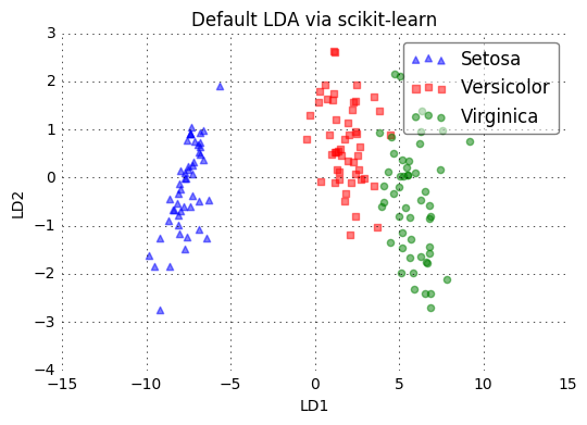
In this contribution we have continued with the introduction to Matrix Factorization techniques for dimensionality reduction in multivariate data sets. In particular in this post, we have described the basic steps and main concepts to analyze data through the use of Linear Discriminant Analysis (LDA). We have shown the versatility of this technique through one example, and we have described how the results of the application of this technique can be interpreted.


